Principal Prediction Patterns
We propose a method for building simple linear
statistical forecast models based on Principal Prediction
Patterns (PPP). The main element of PPP is canonical
correlation analysis (CCA)of a variable at day 0 and the same
variable at a later time ![]() .
.
The PPP appear in pairs, the predictor pattern describing the
initial state and the predictand pattern describing the state at the
forecast time  .
.
If the initial state is  and the state at
 is
is  , then the forecast
is
  with
with  representing the
correlation obtained in the CCA,
  ,
,  the k-th CCA pair,
and
  ,
,  the
k-th. expansion coefficients.
Application to SLP forecast
This analysis was applied to daily Western European air pressure fields from 1900 onwards for lags
![[Graphics:wmo_series_call_9gr11.gif]](Bilder/wmo_series_call_9gr11.gif) .
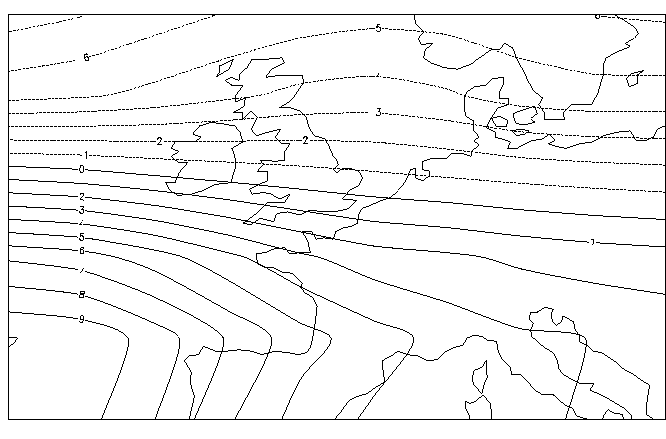
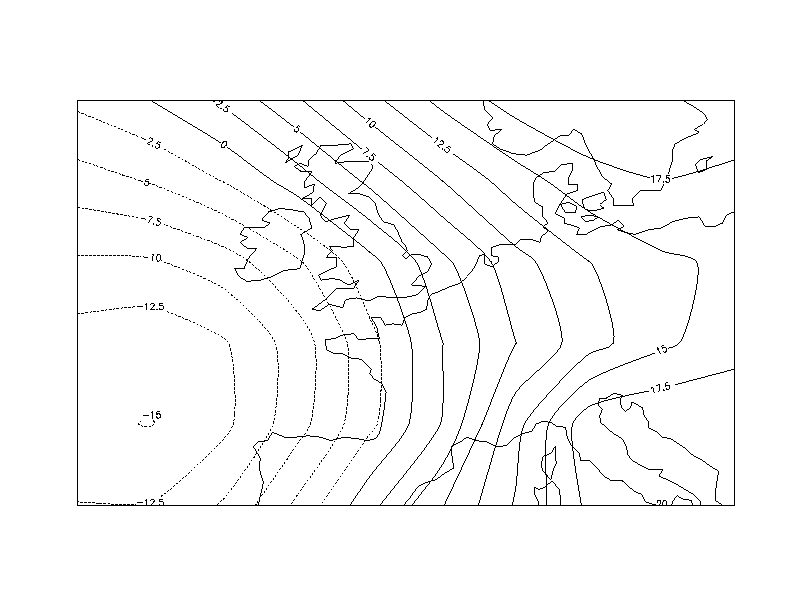
The PPP apppear to remain unchanged with time, as Fig. 1
and Fig. 2 suggest for
.
The PPP apppear to remain unchanged with time, as Fig. 1
and Fig. 2 suggest for
![[Graphics:wmo_series_call_9gr12.gif]](Bilder/wmo_series_call_9gr12.gif) days,
the predictand pattern resembles the predictor pattern. This was noted for all lags. The sum of explained variance
for the first four patterns for
days,
the predictand pattern resembles the predictor pattern. This was noted for all lags. The sum of explained variance
for the first four patterns for
![[Graphics:wmo_series_call_9gr13.gif]](Bilder/wmo_series_call_9gr13.gif) is 0.91.
The correlation of the time coefficients related to the first pattern decreases from 0.9 for one day
forecasts, to 0.66 for three days down to 0.52 for five days.
is 0.91.
The correlation of the time coefficients related to the first pattern decreases from 0.9 for one day
forecasts, to 0.66 for three days down to 0.52 for five days.
Most PPP`s describe only small changes from day 0 to day
![[Graphics:wmo_series_call_9gr1.gif]](Bilder/wmo_series_call_9gr1.gif) , so
that to first order approximation the PPP forecast is a persistence forecast.
An example of a succesfull, non-persistent forecast is the case of January 13, 1901 (Fig. 3 - 5).
Fig. 3
displays the initial slp anomaly distribution which developed to the final state in
Fig. 4 after
, so
that to first order approximation the PPP forecast is a persistence forecast.
An example of a succesfull, non-persistent forecast is the case of January 13, 1901 (Fig. 3 - 5).
Fig. 3
displays the initial slp anomaly distribution which developed to the final state in
Fig. 4 after
![[Graphics:wmo_series_call_9gr14.gif]](Bilder/wmo_series_call_9gr14.gif) days. The anomaly correlation coefficient between the predicted slp anomaly distribution and the
final state (Fig. 5) is 0.93.
days. The anomaly correlation coefficient between the predicted slp anomaly distribution and the
final state (Fig. 5) is 0.93.
For all days in the months DJF of years 1900 to 1990, forecasts with
![[Graphics:wmo_series_call_9gr11.gif]](Bilder/wmo_series_call_9gr11.gif) have been calculated,
Fig. 6 shows the decrease of the mean correlation
coefficient averaged over all forecasts with time lag
have been calculated,
Fig. 6 shows the decrease of the mean correlation
coefficient averaged over all forecasts with time lag
![[Graphics:wmo_series_call_9gr15.gif]](Bilder/wmo_series_call_9gr15.gif) .
The skill is only slightly better than plain persistence.
.
The skill is only slightly better than plain persistence.
The percentage of variance at day 0 explained by the predictor PPP may be used for deriving a measure for the model performance.
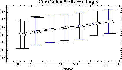
All initial fields are sorted into seven classes of percentage of variance explained by the predictor PPP, with class 1 representing values between 0 and 0.4, while the class seven represents values larger than 0.9. The resulting conditional anomaly correlation coefficients for the PPP forecast as well as for the persistence forecast are shown in Fig. 7. According to Fig. 7, a correlation coefficient of 0.93 agrees to the expected value of 0.56 ± 0.31.
Summary
The PPP analysis identifies the persistent patterns as the most predictable patterns of Western Europe daily air pressure distribution. The PPP forecast is only marginaly better than persistence forecast, yet this method allows us to predict the success of the persistent forecast.
Figures
Fig.1 : predictor PPP for slp anomaly, three day lag, back to the text
Fig.2 : predictand PPP for slp anomaly, three day lag, back to the text
Fig.3 : initial slp anomaly for January 13th. 1901, back to the text
Fig.4 : observed slp anomaly for January 16th. 1901, back to the text
Fig.5 : predicted slp anomaly for January 16th. 1901, back to the text
Fig.6 : mean ± standard deviation of anomaly correlation coefficient vs. time for PPP (diamonds) and persistence (triangles), back to the text
Fig.7 : mean ± standard deviation of anomaly correlation coefficient of a 3 day forecast vs. classes of persentage of explained variance for PPP (diamonds) and persistence (triangles),
back to the text


